MS Excel Data Forms 2007/2010

HOME

If your spreadsheet is too big to manage, and you constantly have to scroll back and forth just to enter data, then a Data Form could make your life easier.  To see what a Data Form is, we will contruct a simple spreadsheet.

But a data form is just a way quick to enter data into a cell.  It is used when the spreadsheet is too big for the screen.  To get a clearer idea of what data form is, try this.

1.  Enter January in Cell A1 of a new spreadsheet.

2.  From A1 to L2, AutoFill the rest of the months to December.

3.  Now, highlight the columns A1 to L1 (click on the letter A and drag to letter L).

4.  On the Home tab in Excel, locate the Cells panel.

5.  On the Cells panel, click the Format item. (In Excel 2013, you will see a menu when you click Format.  From the menu, select Column Width.

6.  From the Format menu, click Width.




7.     Enter a value of say 20 for the column width, and click OK.
8.     Some of your months should disappear from the spreadsheet.

The problem is, if you have to enter data under each month, you 
would have to scroll across to complete the row and then scroll 
back again to start a new row.  Instead of doing this, we will 
create a data form.  You then enter data in the form to complete
a row on your spreadsheet.  No more scrolling back and forth.

In the version of Excel 2007, we have Data Forms have

been hidden.  They used to be sitting on the Data menu.

Now they are not.  In fact, quite a few menu options 

have disappeared in Excel 2007 and Excel 2010.

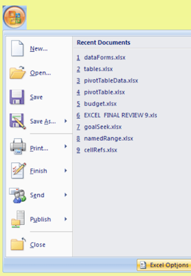
To find Data Forms, click on the office button in the top left of

Excel, for 2007 users.  From the Office button menu, click on 

Excel Options:

For Excel 2010 and 2013 users, click the File tab in the top left. 

From the File menu, click Options.

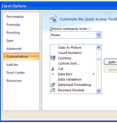
When you click the Excel Options button, you will see this 

dialogue box popping up:

Click the Customization item on the left in Excel 2007.  

In Excel 2010 and 2013 there is a Quick Access Toolbar item. 

Click that instead of Customization.  The idea is that you can 

place any items you like on the Quick Access Toolbar at the top

of the Excel.  You pick one from the list, and then click the Add 

button in the middle.

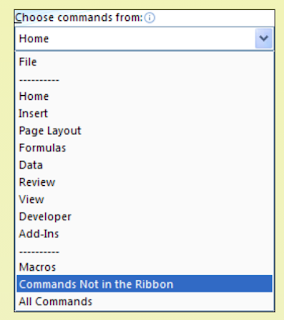
To add the Data Form option to the Quick Access Toolbar, 

click the drop down list where it says Choose Commands 

Form.  You should see this (we have chopped a few options off 

in the image below);

Click on Commands Not in the Ribbon.  The list box 

will change:

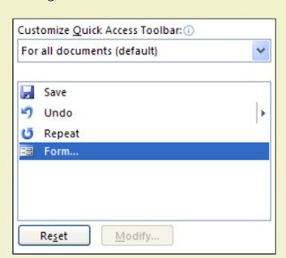
From the Commands Not in the Ribbon list, selec Form.  Now click the Add button in the middle.  

The list box on the right will then look something like this one:

Explore the other items you can add to the 

Quick Access Toolbar.  You might find your favorite 

in there somewhere.

When you click ok on the Excel Options dialogue box, you 

will be returned to Excel.  Look at the Quick Access toolbar, 

and you should see your new item:

Back to the spreadsheet.  Type any number you like in cell

A2, under January.  Then type a number in cell B2 for 

February.  Now highlight the columns A to L again.  This is so 

that Excel will know which is a column heading and which is the

data. 

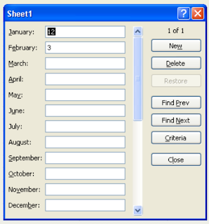
Click the Form item you have just added to the Quick Access 

toolbar:

You should then see this:

All the Columns in the spreadsheet are now showing.

Enter numbers for the other months.  To start a new row in your

spreadsheet, you just click the New button on the right. 

HOME