MS Excel Data Table Part 2

HOME

We will do one more Data Table, just so that you get the hang of things.  This time, we will use a more simple formula than PMT, and we will use Rows instead of Columns.  This is the scenario:

You have 250 items that you want to sell on Ebay.  Your unique selling point in this – All items are only $5 each.  Except, you feel $5 may be a bit expensive for the goods you are selling, what you want to know is how much profit you will make if you reduce your prices to $4.50, how much if you reduce to $4.00, and how much for a reduction to $3.50.  Assume that everything gets sold.

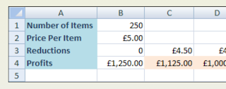
To start creating your table, construct a spreadsheet like the one below.  Make sure that you start on a new sheet.

In cell B1 is the number of items we want to sell (250).  Cell B2 has the original price ($5.00), and the Reductions row has our new values.  Cell B3 has a 0 because there is no reduction for $5.  Row 4 is where our Profits will go.

The formula to work out the profits is simply the Number of Items multiplied by the Price per Item.  So click inside cell B4 and enter the following formula:

=B1 * B2

Your spreadsheet will then look like this:

So, if we manage to sell all our items at $5, we will make $1,250.  We are a bit dubious, though.  Realistically, all our items won’t sell at this price.  Lets use an Excel Data Table to work out how much profit we would make at the other prices.

Again, we put the answer in cell B4 for a reason.  This is because when you want Excel to calculate a Data Table in Rows, the formula must be inserted one Column to the Left of your first new value, and then one Row down.  Our first new value is going in cell C3.  So one column to the left takes us to the B column.  One row down is Row 4.  So the formula goes in cell B4.

Next, click inside cell B3 and highlight to cell E4.  Your spreadsheet should now look like this one:

Excel is going to use our formula in cell B4.  It will then look at the new values on Row 3 (not counting the zero), and then insert the new totals for us.  To create a Data Table then, do the following:

From the Excel menu bar, click on Data.

Locate the Data Tools panel

Click on the “What if analysis” item

Select Data Table from the menu.

Just like last time, you will get the Data Table dialogue box.  The one we want now, though is Row Input cell.  But what is the Input Cell this time?

Ask yourself what you are trying to work out, and what you want Excel to recalculate.  You want to work out the new prices.  The formula you enter was:

=B1 * B2

Excel is going to be changing this formula.  You only need to decide if you want Excel to alter the B1 or the B2.  B1 contains the number of items; B2 contains the price of each item.  Since we are trying to work out the profits, we would get if we change the price, we need Excel to change B2.  So enter B2 for the Row Input cell:

When you click OK, Excel will work out the new profits:

So setting a price of $3.50 per item, you would make $875 profit.  You would make $1000 at $4.00 per item, and $1125 if you sell for $4.50.

HOME