Medical Transcription

MS Excel Tutorial Goal Seek Scenarios Data Table – Part 2 Data Table – Part 1 Add Error Messages Drop-Down Lists Data Forms Template Named Ranges in Excel

HOME Goal Seek is used to get a particular result when you are not too sure of the starting value.  For example, if the answer is 56, and the first number is 8, what is the second number?  Is it 8 multiplied by 7 or 8 multiplied by 6?  You can use Goal Seek to find out.  We will try that example to get you started, and then have go at a more practical example. Create the following Excel spreadsheet: In the spreadsheet above, we know that we want to multiply the number in B1 by the number in B2.  The number in cell B2 is the one we are not too sure of.  The answer is going in cell B3.  Our answer is wrong at the moment, because we has a goal of 56.  To use Goal Seek to get the answer, try the following: From the Excel menu bar, click on Data. Locate the Data Tools panel and then What if Analysis item.  From the What if Analysis menu, select Goal Seek . The following dialogue box appears: The first thin...

HOME Scenarios come under the heading of “What-If Analysis” in Excel.  They are similar to tables in that you are changing values to get new results.  For example, what if I reduce the amount I am spending on food?  How much will I have left then? Scenarios can be saved, so that you can apply them with a quick click of the mouse. An example of a scenario you might want to create is a family budget.  You can then make changes to individual amounts, like food, clothes, or fuel, and see how these changes affect your overall budget. We will see they work now, as we tackle a family budget.  So, create the spreadsheet below: The figure in B12 above is just a SUM function, and is your total debts (=SUM(B3:B10).  The figure in D13 is how much you have left after you deduct all your debts.  In cell D13, then enter =D3 – B12. With only 46 pounds spending money left each month, clearly some changes have to be made.  We will crea...

HOME We will do one more Data Table, just so that you get the hang of things.  This time, we will use a more simple formula than PMT, and we will use Rows instead of Columns.  This is the scenario: You have 250 items that you want to sell on Ebay.  Your unique selling point in this – All items are only $5 each.  Except, you feel $5 may be a bit expensive for the goods you are selling, what you want to know is how much profit you will make if you reduce your prices to $4.50, how much if you reduce to $4.00, and how much for a reduction to $3.50.  Assume that everything gets sold. To start creating your table, construct a spreadsheet like the one below.   Make sure that you start on a new sheet. In cell B1 is the number of items we want to sell (250).  Cell B2 has the original price ($5.00), and the Reductions row has our new values.  Cell B3 has a 0 because there is no reduction for $5.  Row 4 is where our Profits will ...

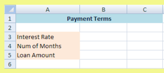
HOME In Excel, a Data Table is a way to see different results by altering an input cell in your formula.  As an example, we are going to alter the interest rate, and see how much a $10,000 loan would cost each month.  The interest rate will be our input cell.  By asking Excel to alter this input, we can quickly see the different monthly payments.  Want to know how much would pay back each month if the interest was 24 percent per year.  But other banks may be offering better deals.  So we will ask Excel to calculate how much we would pay each month if the interest ate was 22 percent a year, 20 percet a year, and 18 percent a year. The formula needed is– PMT ().  Here it is: PMT (rate, nper, pv, fv, type) We only need the first three aguments.  So for us, its just this: PMT (rate, nper, pv) Rage means the interest rate.  The second argument, nper, is how many months you have got to pay the loan back.  The third ar...

HOME Data Validation – Restricting what data go in a cell. You can also restrict what goes in to a cell on your spreadsheet, and display an error message for your users.  We will do this with our comments column.  If users enter too much test, we will let them know by displaying a suitable error box.  Try the following: Highlight the E column on your spreadsheet (the comments column). From the Data Tools panel, click Data Validation to bring up the dialogue box again. From the Allow list, select Text length: When you select Text length from the list, you will see three new areas appear: What we are trying to do is to restrict the amount of text a user can input into any one cell on the Comments column.  We will restrict the text to between 0 and 25 characters. The first of the new areas (Data) is exactly what we want – Between.  For the minimum textbox, just type a 0 (Zero) in there.  For the maximum box, type...

HOME If you have to type the same data into cells all the time, then adding a drop down list to your spreadsheet could be the answer.  In Excel, this comes under the heading of Data Validation. In the example below, we have class of students on a drop down list.  We only have to click a cell in the A column to see this same list of students.  You will see how to do that now.  Here is a picture of your finished spreadsheet. In the image above, we can simply select a student from the drop down list – no more typing.  We can also do the same for the Subject and Grade. So, create the following headings in a new spreadsheet: Cell A1 :  Student Cell B1 :  Subject Cell C1 :  Grade Cell E1 :  Comments We now need some data to go in our lists.  So, type the same data as in the image below.  It does not need to go in the same columns as ours.  But do not type in Columns A, B, C or E: The data...