MS Excel Data Tables Part 1
HOME
In Excel, a Data Table is a way to see different results by altering an input cell in your formula. As an example, we are going to alter the interest rate, and see how much a $10,000 loan would cost each month. The interest rate will be our input cell. By asking Excel to alter this input, we can quickly see the different monthly payments. Want to know how much would pay back each month if the interest was 24 percent per year. But other banks may be offering better deals. So we will ask Excel to calculate how much we would pay each month if the interest ate was 22 percent a year, 20 percet a year, and 18 percent a year.
The formula needed is– PMT (). Here it is:
PMT (rate, nper, pv, fv, type)
We only need the first three aguments. So for us, its just this:
PMT (rate, nper, pv)
Rage means the interest rate. The second argument, nper, is how many months
you have got to pay the loan back. The
third argument, pv, is how much you want to borrow.

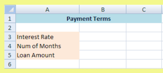
So we will put our starting interest rate in cell B3 (rate),
our loan length in cell B4 (nper), and our last loan amount in cell B5 (pv).

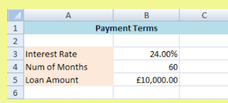
So you need to enter 24.00% in cell B3, 60 in cell B4, and
$10,000 in cell B5.
We will enter our formula now. Click inside cell D2 and enter the following:
=PMT(BE/12, B4, -B5)
Cell B3 is the interest rate. But this is for the entire year. In the formula, we are dividing whatever is
in cell B3 by 12. This will get us a
monthly interest rate. B4 in the formula
is the number of months, which is 60 for us.
B5 has a minus sign before it. It
is a minus figure because it is a debt.
When you press the enter key on your keyboard, Excel should
given you an answer of $287.68.
Now that we have our function in place, we can create an
Excel Data Table. First though we need
to tell Excel about those other interest rates.
It will use these to work out the new monthly payments. Remember, Excel is recalculating the PMT
function. So it needs some new values to
calculate with.
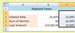
So enter some new values in cells C3, C4, and C5. Enter the same ones as in the image below:
We have put the PMT function in cell D2 for a reason. This is one Row up, and one Column to the
right of our first new interst rate of 22%.
The new monthly payments are going to go in cells D3 to D5. Excel needs the table setting out this way.
So that Excel can work out the new totals, you have to
highlight both the new values and the function you are using.
So highlight the cells C2 to D5. Your spreadsheet should look like this:
As you can see, the cells C2 to D5 are now highlighted. This includes our new interest rate values in
the C column, and our PMT function in cell D2.
We can now creat an Excel Data Table.
This will work out new monthly payments for us. So do this:
From the Excel menu bar, click on Data
Locate the Data Tools
panel
Click on the “Whate if Analysis” item:
When you click on the “What if Analysis” item,
you will see the following menu:
Click on Data Table,
and you will see this small dialogue box:
In the dialogue box, there is only a Row input cell or a Column input cell.
We want Excel to fill downwards, down a column. So we need the second text box on the dialogue
box “Column input cell.” If we were
filling across in rows, we would use the “Row input cell” text box.
So click inside the column input cell box and enter
B3:
Click OK.
When you do, Excel will work out
the new monthly payments:
So if we could get an 18 percent interest rate, our monthly
payments would be $253.93.
If you click inside any of the cells D3 to D5, then look at
the formula bar, you will see this:
{=TABLE(,B3)}
That’s Excel’s way of telling you that a table has
been created, based on the input cell B3.


Comments
Post a Comment